Radiation sources · Microwave tubes · COMSOL simulation
Microwave radiation sources: klystron and traveling-wave tube (TWT)
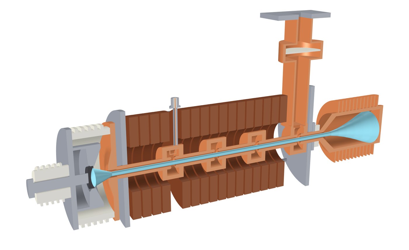
In a klystron or a traveling-wave tube, an electron beam in vacuum gives part of its kinetic energy to an electromagnetic wave and amplifies it. Such tubes are the power amplifiers in radar transmitters, electronic-warfare systems and satellite links. This page shows models I built in COMSOL Multiphysics for both devices: an X-band klystron (9.4 GHz), modeled from the electron gun to the wave leaving through the waveguide, a 6-18 GHz helix TWT and a Ka-band folded-waveguide slow-wave structure.
Klystron: velocity modulation and bunching
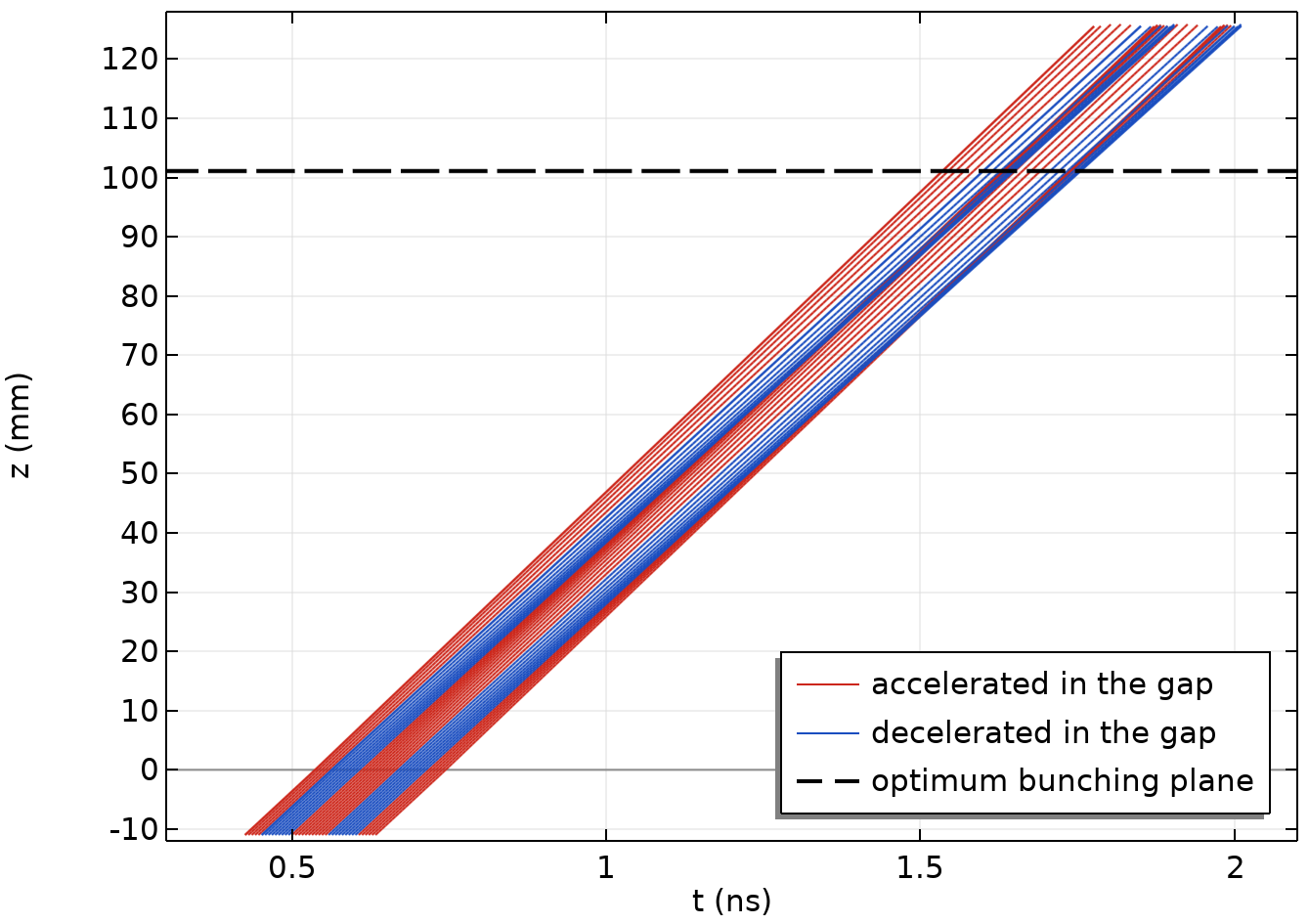
A continuous beam crosses the gap of a resonant cavity. The alternating gap voltage speeds some electrons up and slows others down, and in the drift region the fast electrons catch up with the slow ones: the beam gathers into bunches that repeat at the signal frequency. The output cavity sits where the first harmonic of the beam current peaks, and the bunched current excites a field there that leaves through the waveguide.
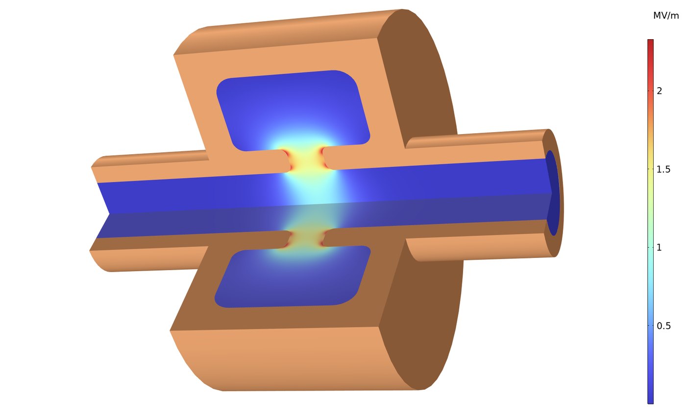
The cavity is solved as a 2D axisymmetric model, and a tuning script adjusts its radius until the fundamental mode sits at 9.4 GHz. Wall losses come from a copper impedance boundary condition.
- Q0 of 4,080 with copper walls
- R/Q of 77 Ω (circuit convention, V²/(2ωU))
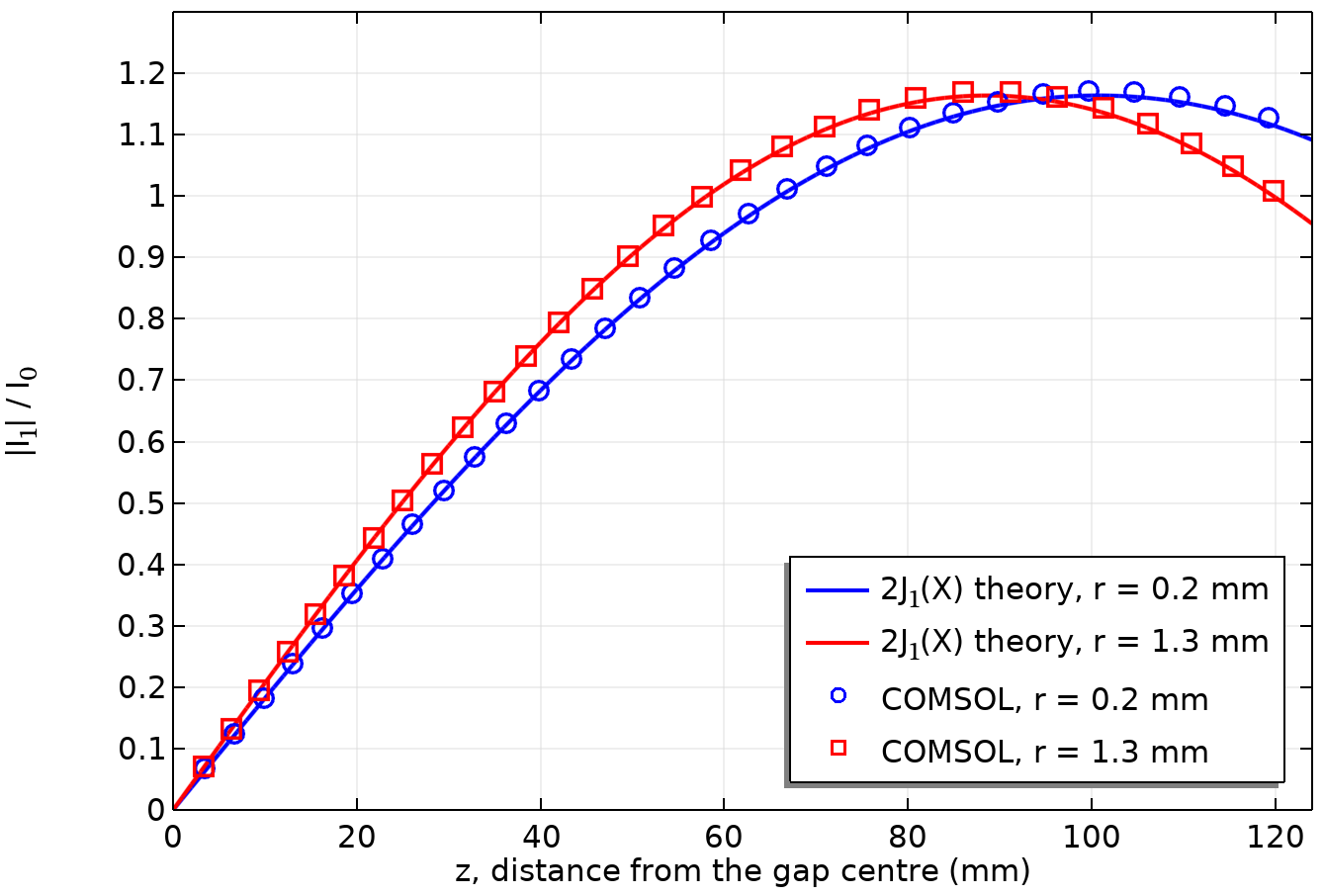
The computed cavity mode drives the particle tracing directly as the modulating field. Space charge is left out, so the field-particle coupling can be compared with ballistic theory: the distance to maximum bunching, about 93 mm from the gap averaged over the beam, matches theory within 0.3%, and the peak first harmonic of the beam current is 1.17 times the DC current, compared with 1.16 in theory.
Output cavity and waveguide
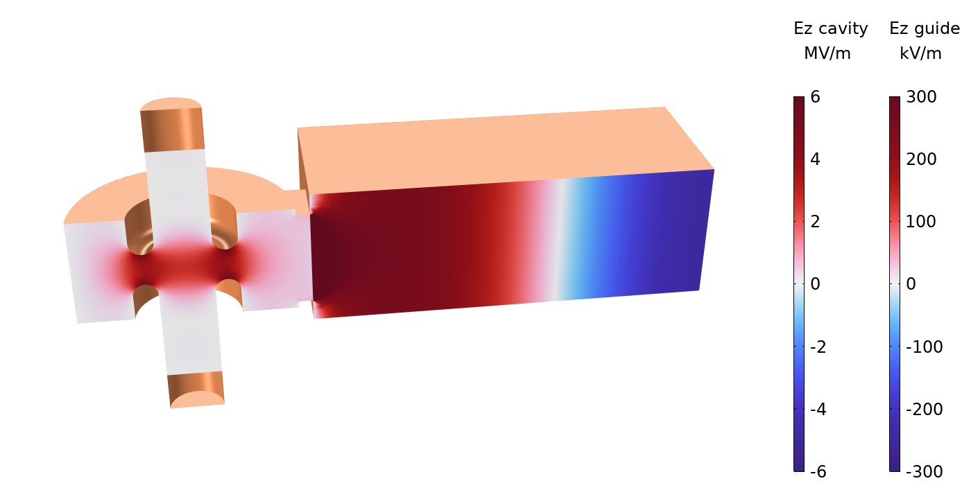
The output cavity couples through an iris into a WR-90 waveguide. An eigenfrequency solution of the cavity together with the waveguide gives a complex frequency, and from it the loaded quality factor and the external Q, which sets how fast the energy delivered by the bunches leaves into the waveguide.
- Loaded quality factor of 368, from the complex eigenfrequency
- External Q of about 400, compared with an unloaded Q0 of the output cavity of about 4,060 (wall losses): about 90% of the power the bunches deliver to the cavity leaves into the waveguide
Electron gun
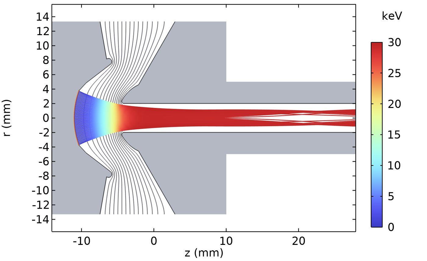
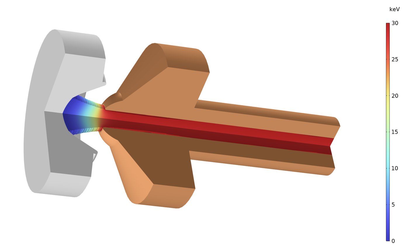
A concave spherical cathode emits a space-charge-limited current (Child's law), and the focus electrode and anode shape the field so that the beam converges into a 2 mm-radius beam tunnel. Field and trajectories are iterated until the emitted current settles. The gun emits 4.16 A at 30 kV (perveance 0.80 µP) with an average cathode loading of about 9 A/cm², and the beam reaches a waist of 1.1 mm radius about 12 mm past the anode lip. Without a magnetic field the beam hits the beam-tunnel wall about 20 mm after the waist, which is why a focusing solenoid surrounds it in the klystron.
Traveling-wave tube: helix slow-wave structure
In a traveling-wave tube the beam and the wave travel together, and the electrons give energy to the wave while they move slightly faster than its phase velocity. The helix slows the wave down: the signal runs along the metal tape at nearly the speed of light, and along the axis it advances about eight times slower. The phase velocity changes little with frequency, which is why a helix amplifier covers a band as wide as 6-18 GHz.
In the 3D model the axial wavelength at 12 GHz is 3.03 mm, compared with 25 mm in free space. The phase velocity, 0.121 of the speed of light, matches a beam of about 3.8 kV.
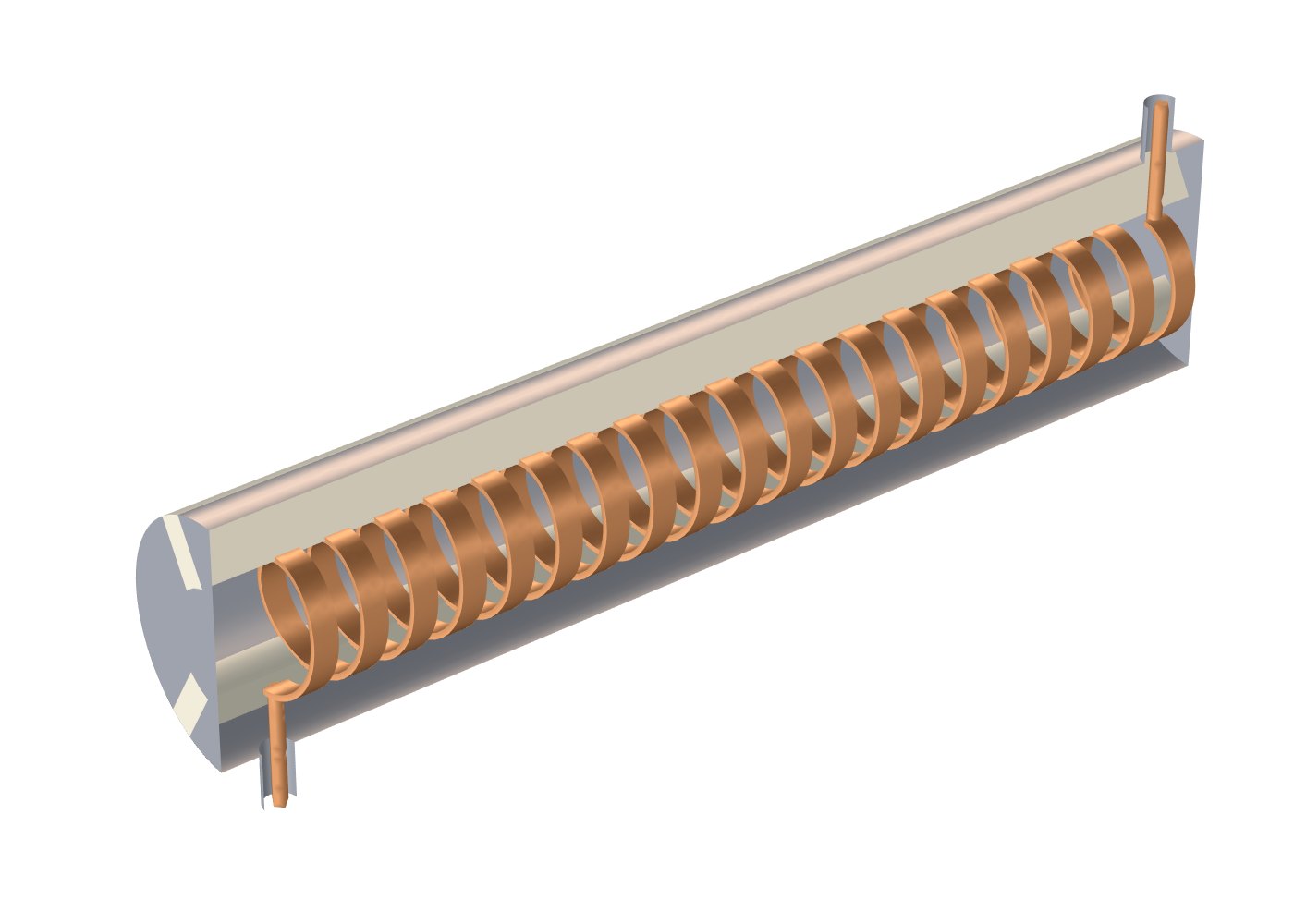
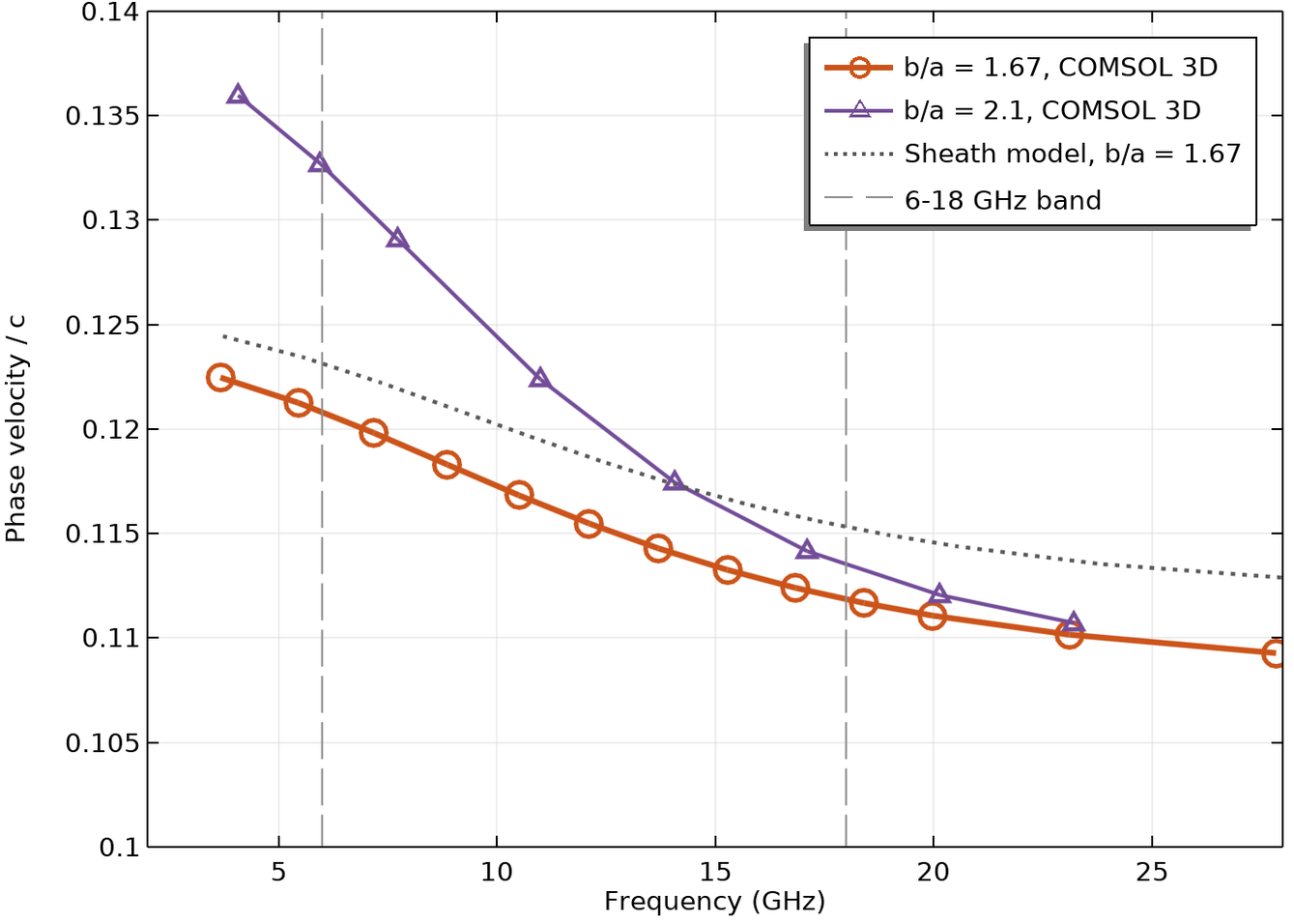
One unit cell of the helix with periodic (Floquet) boundary conditions is enough to compute the dispersion curve and the interaction impedance across the band. The cell chosen for the band is a smaller helix (0.6 mm radius, compared with 0.8 mm in the 3D model) in a closer barrel. In this cell the phase velocity falls from 0.121 to 0.112 of the speed of light between 6 and 18 GHz (±3.8%), and a 3.45 kV beam is synchronous with the wave at 12 GHz. A metal barrel close to the helix flattens the dispersion: with a wider barrel the variation grows to ±7.8%.
Ka-band folded waveguide
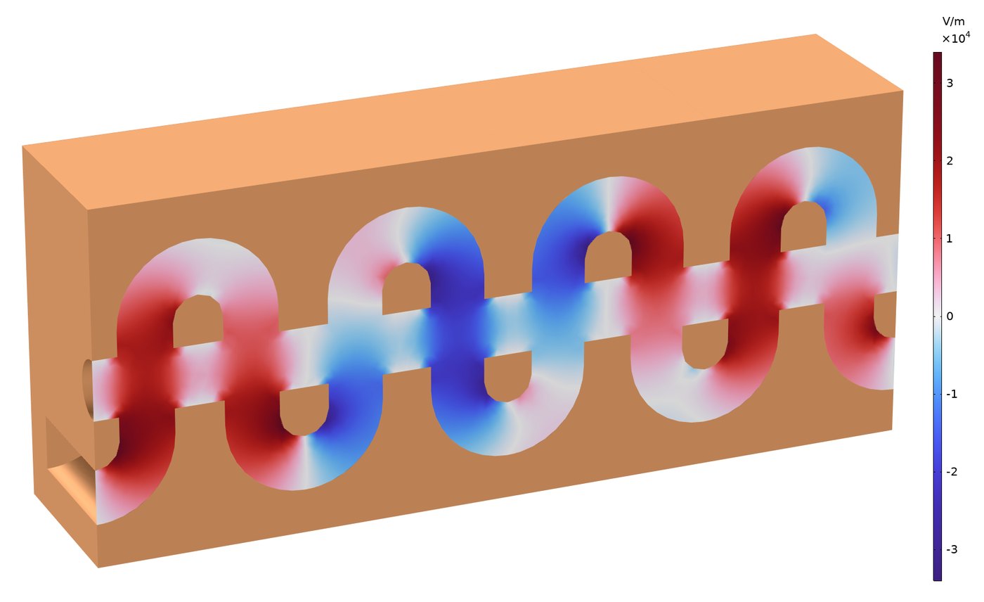
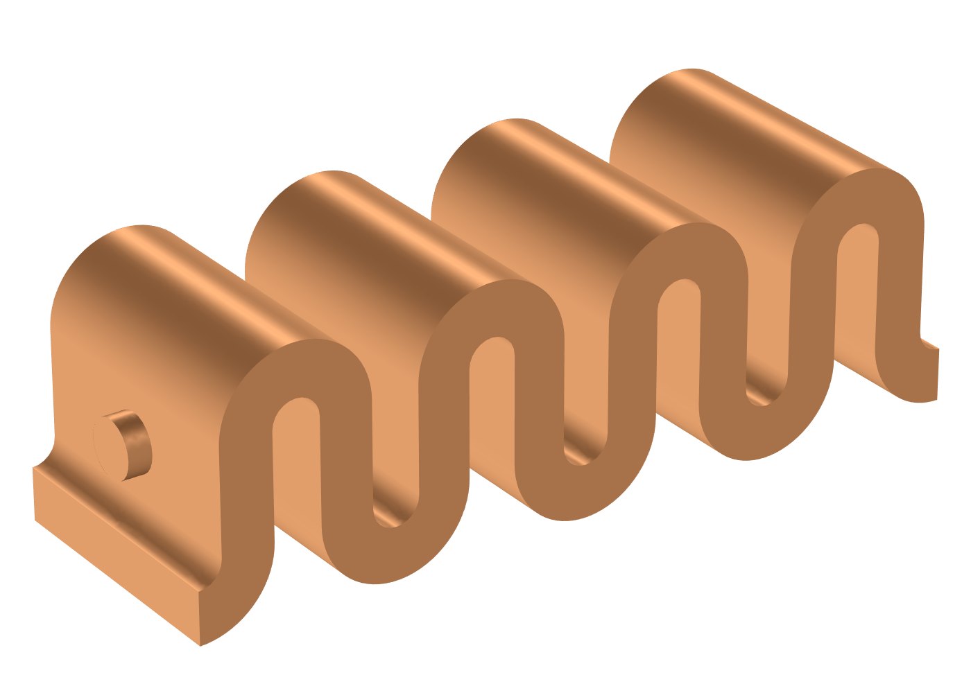
At higher frequencies the helix becomes very small and limited in power, and the slow-wave structure is made of a rectangular waveguide that folds back and forth across the beam tunnel. The wave follows the serpentine path while the beam crosses it at every fold, twice per period, so along the axis the wave advances slower than light. The structure is all metal and removes heat better than a helix held on ceramic rods. The model is a unit cell with periodic boundary conditions, solved around 35 GHz.
What the models demonstrate
- Eigenfrequencies of resonant cavities with wall losses
- A computed RF field as input to relativistic particle tracing
- Space-charge-limited emission and Pierce-gun beam optics
- Periodic boundary conditions for dispersion and interaction impedance
- Coupling to waveguide and coaxial lines, scattering parameters
- Full 3D geometry and animations rendered in COMSOL
My PhD dealt with terahertz generation in free-electron devices. Research on undulator radiation from electron bunches and on acceleration in helical undulators is on the accelerators page, and more COMSOL examples are on the simulations page.
For technical questions and research collaboration: nezahb@ariel.ac.il